Linear Regression
Task Formulation
N data points where where there are certain features that are all numeric.
where for all
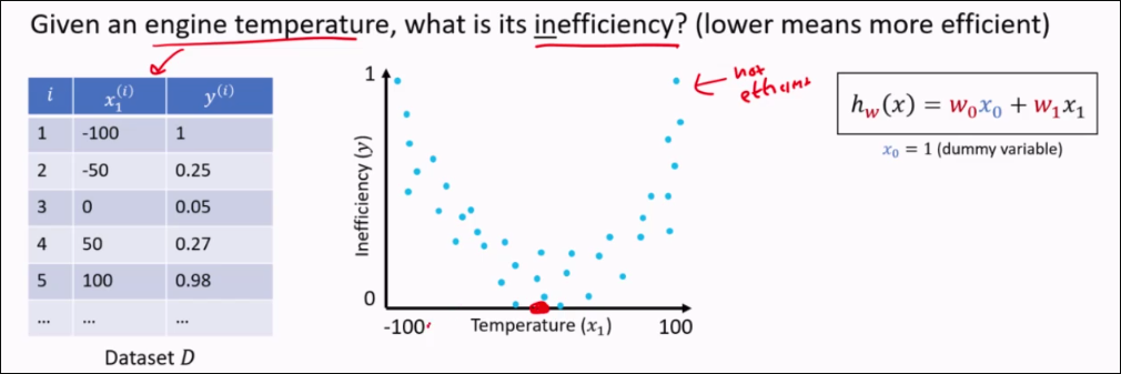
To find a function that predicts the target y for a given x, is called regression
Linear Models
Where
Shorthand:
A model is linear as long as it is some linear combination of weights - variables can be squared, even.
There are infinitely many linear models that could represent the relationship between input x and output.
We want a linear model with the lowest loss on the data - commonly use mean squared error
TODO: Include mean squared error loss here.
Question:
Select The correct statements
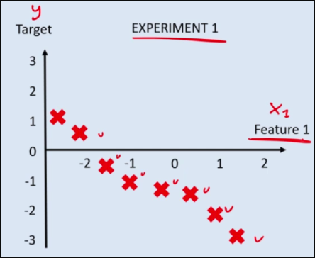
For EXPERIMENT 1, the best linear model will have $ w_0 > 0 $
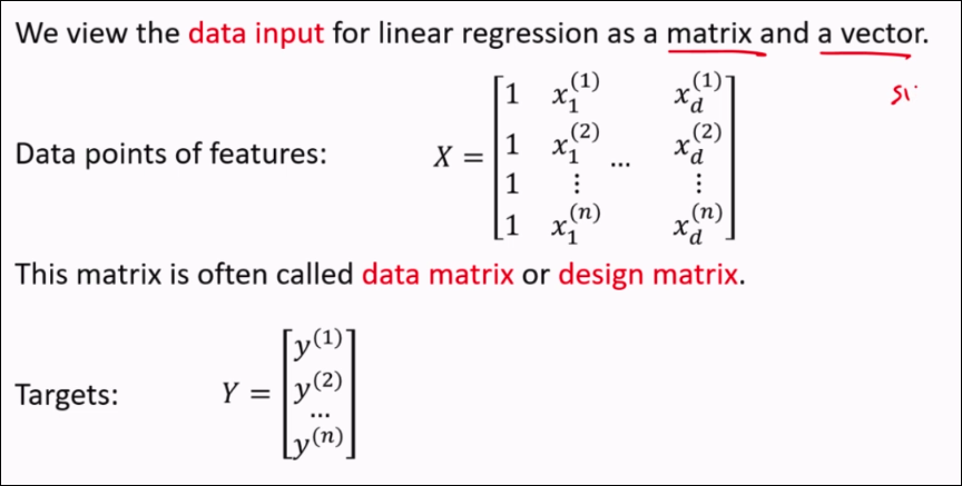
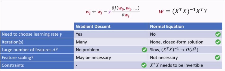
Learning via Normal Equations
Viewing input/output as a matrix
The Normal Equation
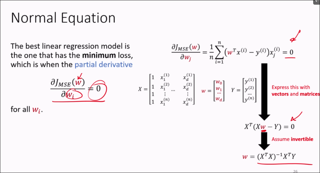
However, the normal equation has its problems:
- The cost of the normal equation is d^3 (for inverting the matrix)
- It will not work if
is not invertible - It will not work for non-linear models
Learning via Gradient Descent
- Start at some
- Update
with a step in the opposite direction of the gradient:
- Learning rate
is a hyperparameter that determines the step size. - Repeat until termination criteria is satisfied.
Multi-Variable Gradient Descent
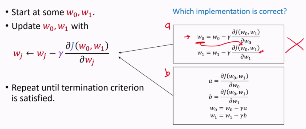
You have to update both at the same time, if not the first operation spoils the result of the 2nd equation
Gradient Descent - Analysis
Theorem: MSE loss function for a linear regression model is a convex function with respect to the model's parameters.
Definition: Linearly dependent features: A feature is linearly dependent on other features, if it is a linear combination of the other features. E.g.
Theorem: If features in the training data are linearly independent, the function (MSE + Linear model) is strictly convex
And thus,
Theorem: For a linear regression model with a MSE loss function, the Gradient Descent algorithm is guaranteed to converge to a global minimum, provided the learning rate is chosen appropriately. If the features are linearly independent, then the global minimum is unique.
A problem with Gradient Descent
Let's say we have j(w) given data 2 datapoints with 2 dimensions and 1 target variable:
Then, it's gradient is given:
Gradient descent update is then given:
This causes a problem, because we then have the gradient given by the graph:
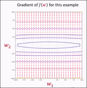
The gradient change for
How to fix this?
- Min-max scale the features to be within [0, 1]
- Standardize the data based on the mean
- Use a different learning rate for each weight
Other problems in Gradient Descent
Slow for large datasets, since the entire dataset must be used to compute the gradient.
May get stuck at a local minimum/plateu on non-convex optimization.
Use a subset of training examples at a time (Mini-batch GD). Cheaper/Faster per iteration.
Stochastic Gradient Descent - select one random training example at a time.
Linear Regression Summary
Feature Transformation
Take a d-dimensional feature vector and transform it into an M-dimensional feature vector, where usually
Where,
- The function
is called a feature transformation/map - The vector
is called the transformed features
Theorem: The convexity of linear regression with MSE is preserved with feature transformation.
TODO: Interpretation of that partial derivative shit (how to perform gradient-descent related) What a minimizer is MSE/MAE tutorial? LR. ACC/PREC/F1 Score