Machine Learning

Learning Agents

Rather than solve the problem explicitly, construct an agent that learns a function to identify patterns in the data and make decisions.

Supervised Learning

Involves:

• Data: A set of input-output pairs that the model learns from
  • Assume it represents the ground truth
• Model: A function that predicts the output based on the input features.
• Loss: A function that is used by a learning algorithm to assess the model's ability in making predictions over a set of data.

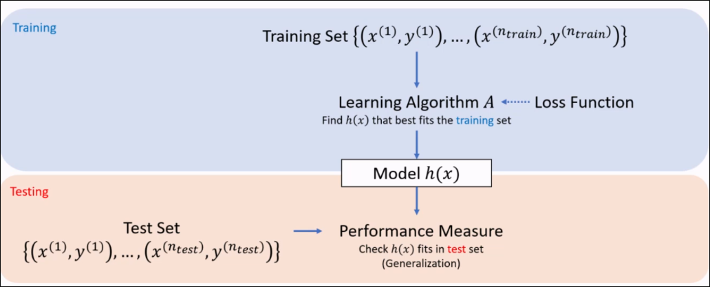
A learning algorithm is an algorithm that seeks to minimize the loss of a model over a training dataset. Used in the training phase.

After training, we usually test on an unseen test set. This is used to evaluate the model using various measures. This measures the generalization of the model.

Tasks in Supervised Learning

Classification

• Objective: predict a discrete label - cat or dog?
• Output is a categorical value
• Cancer prediction, Spam detection

Regression

• Objective: predict a continuous numerical value based on input features.
• The output variable is a real number

Data formulation

A dataset is represented as:

$$(x^{(i)}, y^{(i)})$$

• $x^{(i)} \in \Reals^d$ is the input vector of $d$ features of the $i^{th}$ data point.
  • In general, $x^{(i)}$ can be a multi-dimensional array of features

• $y^{(i)}$ is the label for the $i^{th}$ data point.
  • Regression: $y^{(i)} \in \Reals$ for regression
  • Classification: $y^{(i)} \in {1, 2, .., K}$ for classification with $K$ classes.

Dataset $D$ with $n$ examples can be represented as:

$$D = {(x^{(1)}, y^{(1)}), (x^{(2)}, y^{(2)}), ..., (x^{(n)}, y^{(n)})}$$

Model

Refers to a function that maps from input to outputs: $h:X \rightarrow Y$. $h(x)$ should best predict the outputs given x.

Performance Measure & Loss

Performance Measure & loss functions take in a dataset $D$ and a model $h$ and returns a number representing how well $h$ predicts the mapping.

• Performance measure: is a metric that evaluates how well the model performs on a task. Used in evaluation/testing.
• Loss function: Quantifies the difference between the model's predictions and the true outputs. It's used by the model the guide learning to reach the optimal outcome.

Regression

Mean squared error (MSE)

$$MSE = \frac 1 n \sum_n^{i=1} (\widehat{y}^{(i)} - y^{(i)})^2$$

Mean squared error (MSE)

$$MAE = \frac 1 n \sum_n^{i=1} |(\widehat{y}^{(i)} - y^{(i)})|$$

$\widehat{y}$ represents the prediction of the model. These metrics can also be used as loss functions.

Classification

Accuracy

$$Accuracy = \frac 1 n \sum_{i=1}^n 1 (\widehat{y}^{(i)} = y^{(i)})$$

Confusion Matrix

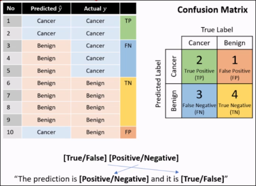
Measure TPR, TNR, FPR, FNR, etc.

Learning Algorihtms

A learning algorithm A takes in a training set $D_{train}$, consisting of pairs, and seeks to find a model $h$ to approximate the true relationship between inputs and outputs. They can utilize loss functions to guide them.

Decision Tree

A decision tree is a model that outputs a categorical decision or prediction. A decision is reached by sequentially checking the attribute value at each node, starting from the root until a leaf is reached.

There generally exists multiple distinct DTs that are all consistent with the training data.

We prefer COMPACT decision trees, are they're less likely to be consistent with training solely due to chance

Entropy

Entropy quantifies the uncertainty or randomness of a random variable.

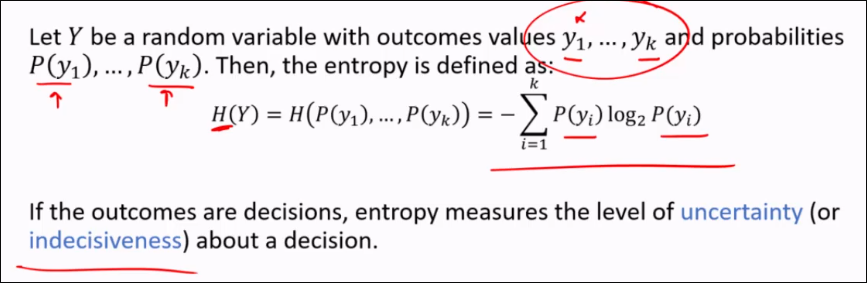
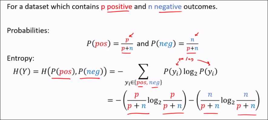
In binary outcomes, entropy is:

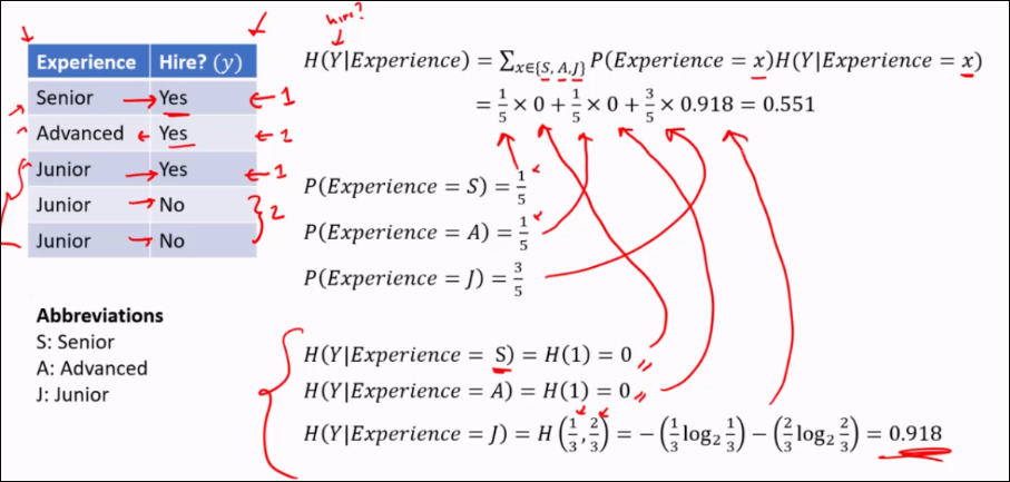
Specific Conditional Entropy

Specific conditional entropy H(Y|X=x) is the entropy of a random variable Y conditioned on the discrete random variable X.

Simply fix the DRV, then calculate entropy as before.

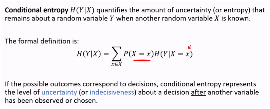
Conditional Entropy

It is simply the Expected Value - multiply the probability of a feature with the specific conditional entropy for each category x in X.

Information Gain

Information gain is a measure of the reduction in uncertainty about a particular decision after knowing the value of a specific variable.

$$IG(Y;X) = H(Y) - H(Y|X)$$

Decision Tree Learning

Top-down, greedy, recursive algorithm.

• Top-down: Build the decision tree from the root.
• Greedy: At each step, choose the locally optimal attribute to split, such as based on immediate information gain, without considering future splits.
• Recursive: For each value of a chosen attribute, use DTL again on corresponding subset of data.

Stopping Criteria:

• No more data or attributes
• All data predicts the same class

DTL - Functions

• choose_attribute(attributes, rows)

  • Accepts a set of attributes (columns) in the data, and the rows containing the data points.
  • Computes gain of each attribute
  • Returns the attribute that has highest information gain

• majority_decision(rows)

  • Accepts the table rows containing the data points.
  • Returns the most common decision in the data points.

DTL - Base Case

1. No data available -> return default
2. Same classification for all rows -> return that classification
3. attributes is empty -> Take majority decision

def DTL(rows, attributes, default):
  if rows is empty; return default
  if rows have the same classification:
    return classification
  if attributes is empty:
    return majority_decision(rows)

  best_attribute = choose_attribute(attributes, rows)
  tree = a new decision tree with root best_attribute
  for value of best_attribute:
    subrows = {rows with best_attribute = value}
    subtree = DTL(
              subrows,
              attributes - best_attribute,
              majority_decision(rows)
            )
    add subtree as a branch to tree with label value
  return tree

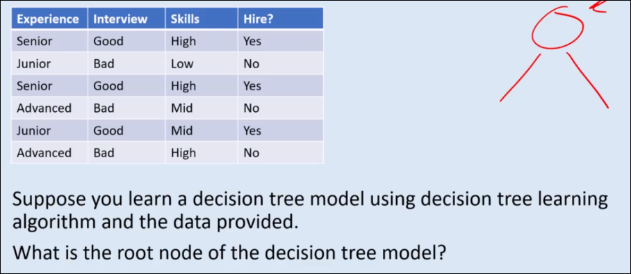
Question:

DT analysis

Theorem (Representational completeness of Decision Tree)

For any finite set of consistent examples with categorical features and a finite set of label classes, there exists a decision tree that is consistent with the examples.

But this is problematic. The DT then is prone to noise or outliers in excessively complex DTs - overfitting.

DT pruning

Pruning refers to the process of removing parts of the tree. The goal is to produce a simpler, more robust tree that generalizes better.

Common pruning methods:

• Max depth: limits the maximum depth of the DT.
• Min-sample leaves: Set a minimum threshold for the number of samples required to be in each leaf node.